


Introduction
Inter-Integrated Circuit (I2C) and Controller Area Network (CAN) are two widely used communication protocols in embedded systems. Both allow microcontrollers and peripherals (like sensors or other ICs) to exchange data, but they differ significantly in design and capabilities. This report provides an overview of each protocol and a detailed comparison focusing on performance metrics such as data rate, bus length, fault tolerance, and power consumption. The discussion is tailored for beginner to intermediate readers in embedded systems, with examples relevant to common platforms (STM32, Arduino, Raspberry Pi) kept general. By understanding the strengths and trade-offs of I2C and CAN, developers can choose the appropriate bus for their application needs.
I2C Protocol Overview
I2C is a simple two-wire, synchronous serial bus designed for short-distance communication between chips on the same board. It uses one line for serial data (SDA) and one for serial clock (SCL), both of which are open-drain (open-collector) signals that require pull-up resistors. In an I2C bus, a device configured as the master controls the clock and initiates communication, while one or more slave devices respond. Notably, I2C supports multiple masters arbitrating the bus (multi-controller capability), though in practice one master is common. Each slave device has an address, and communications are addressed to specific targets on the shared bus.
I2C’s hardware simplicity is one of its biggest advantages. Only two wires are needed to connect up to dozens of devices (the 7-bit addressing allows up to 127 addresses, although practical limits are lower) on the same bus. This minimal wiring and the open-drain design help avoid driver conflicts on the bus (devices only pull lines low, never drive them high, which prevents electrical contention). However, I2C was intentionally created for intra-board communication and lower data rates. Standard I2C modes have moderate speeds: 100 kbit/s in standard mode, 400 kbit/s in Fast Mode, and up to 3.4 Mbit/s in High-Speed Mode (with a newer ultra-fast mode of 5 Mbit/s for unidirectional use). These bit rates are sufficient for many sensor readings or configuration tasks, but are lower than what some other interfaces (like SPI or CAN) can achieve.
Because I2C uses pull-up resistors and a wired-AND signaling scheme, the physical bus length and capacitance are limited. The I2C specification recommends a maximum bus capacitance of about 400 pF; beyond this, signal rise/fall times become too slow and integrity degrades. In practical terms this restricts I2C to just a few meters of cable at most (and much shorter lengths at high speeds). Typically, I2C is used on a single circuit board or between modules in close proximity, not for long cables or noisy environments. I2C also has very minimal built-in error handling – after each 8-bit byte transmitted, the receiver sends a single ACK/NACK bit to acknowledge reception. Aside from this acknowledgment, I2C has no error correction codes or retransmission mechanism at the protocol level. If data is corrupted or a device misbehaves (for example, a stuck line), the bus can hang or deliver wrong data unless the master or software takes action to recover. Despite these limitations, I2C’s simplicity and low overhead make it ideal for board-level communication with sensors, memory chips, display controllers, etc., and virtually all microcontroller families (including STM32, Arduino AVR, and Raspberry Pi’s SoC) include at least one I2C interface for such purposes.
CAN Protocol Overview
CAN is a robust differential bus protocol originally developed for automotive applications, where reliability in harsh environments is critical. Unlike I2C’s simple two-wire open-drain scheme, CAN uses a twisted-pair of wires (CAN High and CAN Low) driven in a differential fashion. All nodes on a CAN bus broadcast messages to the network, and every node can listen or transmit – it is a true multi-master network with built-in arbitration to resolve collisions. A key aspect of CAN is that communication is message-based: each frame transmitted contains a message ID (identifier) and up to 8 bytes of data (in the classical CAN 2.0 standard). Rather than addressing a specific receiver, the ID denotes the content or priority of the message, and any node interested in that ID will process it. This makes CAN very flexible for systems with many microcontrollers (e.g. in a car) sharing data on one bus.
The CAN protocol was designed from the start with robustness and fault tolerance in mind. It employs a number of built-in error detection mechanisms and a fault confinement system. For example, each CAN message includes a Cyclic Redundancy Check (CRC) for error detection, and all receivers send a collective acknowledgment bit if they received the frame correctly. If any node detects a defect in the frame (such as a CRC mismatch or a formatting error), it will transmit an error flag that causes the frame to be discarded and automatically retried. Each CAN controller keeps internal error counters and will isolate itself (enter a “bus off” state) if it misbehaves or experiences excessive errors, thereby preventing one faulty node from bringing down the entire network. This level of error handling and fault containment is a major difference from I2C. Engineers often choose CAN for safety-critical or noisy environments specifically for these reliability features.
PICAN CAN Bus FD Board With Real-Time Clock For Raspberry Pi
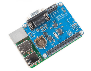 The PiCAN CAN‑Bus FD Board with Real‑Time Clock, designed for the Raspberry Pi, integrates a Microchip MCP2517FD CAN‑FD controller and MCP2562FD transceiver—fully compliant with ISO 11898‑1:2015—for reliable flexible data‑rate CAN communications via SPI. It supports both classic CAN (up to 1 Mbps arbitration rate) and CAN FD (with data-phase speeds up to 8 Mbps), making it suitable for high-performance automotive and industrial networking. The board also features a PCF8523 RTC module with battery backup for accurate timekeeping, and can power the Pi via onboard SMPS from either a DB9 connector or screw terminal. Linux support is seamless through SocketCAN, enabling easy development in C or Python. More information…
In terms of performance, standard CAN (CAN 2.0) supports data rates up to 1 Mbit/s on the bus. The achievable length of the bus is inversely related to the data rate: for example, a CAN bus can be about 40 m long at 1 Mbit/s, but if the speed is reduced to 125 kbit/s, the bus length can extend to around 500 m (this is a common trade-off in CAN networks). Newer enhancements like CAN FD (Flexible Data Rate) allow higher throughput – CAN FD nodes can transmit the data portion of the frame at higher bit rates (up to around 5–8 Mbit/s in practice) and can carry up to 64 bytes of user data per frame. These improvements require CAN FD-capable hardware but remain backward-compatible in the arbitration phase. Whether using classical CAN or CAN FD, the bus still only requires a pair of wires and can support a large number of nodes (often dozens of devices) on the network. However, unlike I2C, implementing CAN on a microcontroller typically requires an external CAN transceiver chip (to convert the microcontroller’s logic-level CAN controller signals to the differential voltages on the bus). Many microcontrollers – for instance, numerous STM32 models – include a built-in CAN controller peripheral, but you still need a transceiver chip (like the MCP2551 or SN65HVD230, etc.) to interface with the bus lines. some high-performance Arduino variants (or shields) and add-on boards for Raspberry Pi provide this hardware so those platforms can use CAN. This extra hardware and configuration reflect the fact that CAN’s physical layer is more complex than I2C’s, but they also enable CAN’s robustness.
Detailed Comparison of I2C vs. CAN
Below is a point-by-point comparison of I2C and CAN, highlighting key differences in data rate, bus length, fault tolerance, and power usage, particularly in the context of embedded systems and microcontroller use.
Data Rate and Throughput
-
I2C Speed: I2C was designed for relatively low to moderate data rates. Standard I2C runs at 100 kbps, with a commonly used Fast Mode at 400 kbps. Some devices and microcontrollers support Fast Mode Plus at 1 Mbps, and High-Speed Mode at 3.4 Mbps (with a very limited ultra-fast mode of 5 Mbps). These clock rates directly translate to raw bit throughput on the bus; however, the effective data throughput is lower after accounting for protocol overhead (address bytes, acknowledgments, etc.). For example, each transmitted byte incurs an ACK bit, and communications often include addressing and register bytes, so you never get to use the full clock rate purely for payload. Nevertheless, I2C’s speed is sufficient for many sensor readings, configuration registers, or modest data transfers in embedded devices. Its strengths lie in simplicity rather than high bandwidth.
-
CAN Speed: CAN in its classical form supports up to 1 Mbps on the bus. Unlike I2C, CAN frames carry a fixed maximum payload of 8 bytes, so sending large amounts of data requires multiple frames. Even so, CAN can be considered a higher-speed protocol in contexts like automotive sensor networks, where messages are typically a few bytes and need to be broadcast quickly. The CAN FD extension increases the payload size (up to 64 bytes) and allows switching to higher bit rates (several Mbps) during the data portion of a frame. This means CAN FD can achieve much higher throughput than classical CAN when supported. It’s worth noting that because CAN uses a priority-based arbitration (where lower ID numbers have higher priority), a stream of high-priority messages could delay lower-priority ones under heavy load. But in general, CAN is efficient for periodic real-time data because messages that get through are checked and ACKed by all receivers. In summary, standard CAN provides reliable medium-speed communication (1 Mbps) suitable for many microcontroller networks, and with CAN FD it can approach the data rates of some simpler serial buses while still maintaining its robustness.
Arduino-Based ECU Development Board With Dual CAN Bus Interface
 This development board is built around the Arduino Due (Atmel SAM3X8E ARM Cortex-M3, 84 MHz, 512 KB flash, 96 KB SRAM) and adds two fully wired CAN bus ports via integrated transceivers, enabling robust interfacing with dual CAN networks. It supports a wide input voltage range (7–36 V DC), making it ideal for vehicle and industrial environments, and includes switchable termination resistors and LED activity indicators for both CAN channels. The board is compatible with standard Arduino shields and leverages the Arduino ecosystem—including software libraries for CAN, OBD-II, and SAE J1939—making it ready for rapid prototyping of CAN or SAE J1939 applications like gateways, data loggers, or telematics systems. More information…
Bus Length and Network Topology
-
I2C Bus Length: I2C is intended for short-range communications, such as on a single PCB or within a device. The limitation comes from the electrical characteristics: I2C lines are open-drain with pull-ups, so the bus behaves like an RC circuit with the total capacitance of all nodes and wiring. The official limit is 400 pF on the bus, which corresponds to only a few meters of wire (at most) even at 100 kHz speeds. In practice, I2C works best over just centimeters or tens of centimeters. Longer cables introduce more capacitance and are more prone to noise, causing slower edges and possible communication errors. Some designs do extend I2C over a meter or two using lower clock speeds or special bus extender chips, but generally if you need to span more than a couple of boards or a wiring harness, I2C is not the best choice. All devices on an I2C bus share the same two wires in a wired-AND bus topology, and you typically need a common ground reference. The number of devices is theoretically limited by addresses (127 in 7-bit addressing) and practically by capacitance and address conflicts. In summary, I2C connects a handful of chips in close proximity – it’s not suited for networking across a vehicle or building.
-
CAN Bus Length: CAN is designed for longer distances and distributed systems. Using a differential pair and terminating resistors at the ends of the bus, a CAN network can span a much greater distance than I2C while maintaining integrity. For example, a high-speed CAN bus (1 Mbps) can reliably operate around 40 meters in length, and by reducing the bit rate to 125 kbps, the bus length can extend to roughly 500 m. This ability to trade speed for distance is a key advantage of CAN in large installations (such as vehicles, factories, or building automation). The differential signaling cancels out common-mode noise and allows for ground potential differences between nodes, which is essential in electrically noisy or large systems. In terms of topology, CAN is usually wired as a single linear bus (with short stubs to individual nodes) with up to 120 Ω termination at each end. It can support many nodes (the protocol doesn’t set a hard limit on node count; practical limits of 30–100 nodes or more can be connected, depending on the transceivers and bus loading). Every node just taps into the two-wire bus. This makes CAN well-suited to networking multiple microcontrollers over a vehicle or across modules in an industrial setup. In short, bus length and area coverage is a major differentiator: CAN can connect devices across rooms or vehicles, whereas I2C is confined to within a device or small module.
Fault Tolerance and Reliability
-
I2C Fault Tolerance: Reliability in I2C largely depends on the system design and software, because the protocol itself provides minimal fault handling. The only built-in check is the ACK/NACK bit after each byte, which tells the transmitter if the receiver got the byte or not. If a device is not present or a byte was corrupted enough that the receiver’s address didn’t match, you’ll get a NACK. However, I2C has no mechanism like a checksum to detect data corruption within a byte, and no automatic retry – it’s up to the master’s software to notice missing ACKs or other anomalies and decide to attempt a retransmission. A common failure mode in I2C is a “stuck bus”, where a misbehaving device holds a line (SDA or SCL) low due to a fault or a missed stop condition. In such cases, the bus can lock up and there is no standard hardware recovery. The master may try to toggle SCL or issue clock pulses to free a stuck slave, or ultimately reset power to devices to clear the condition. But fundamentally, I2C hardware won’t recover on its own – it relies on the system design for fault recovery (e.g. having timeouts and the ability to reset peripherals). I2C is also sensitive to electrical noise; a spurious pulse on SCL or SDA can upset the state of the bus (since I2C doesn’t use differential signals or robust error checking). Good practice in I2C designs includes using shielding or twisted pairs for longer runs and avoiding hot-plugging I2C devices (to prevent glitches). In summary, I2C is not very fault-tolerant by itself – it assumes a relatively clean environment and well-behaved devices. Any required reliability (for instance, in a sensor network) must be added by higher-level protocols or careful design.
-
CAN Fault Tolerance: CAN was fundamentally built with reliability and fault tolerance in mind. It has multiple layers of error detection: bit monitoring (each transmitter listens to the bus to ensure the bit value it put out actually appears), bit stuffing rules (which ensure a minimum number of signal edges and can detect some errors), frame checks for format errors, ACK checks, and a CRC for each frame’s data. If any node detects an error via these mechanisms, it sends an error frame (a special sequence that disrupts the bus), causing all nodes to discard the current message. The transmitter will then automatically retry sending the message until it succeeds (or a maximum error limit is reached). This means transient errors (noise-induced bit flips, for example) are corrected by automatic retransmission. Moreover, CAN nodes implement an error counter system: nodes that experience frequent errors will first enter a passive state (where they don’t actively flag errors, to avoid spamming the bus) and if problems continue, they go into a bus-off state, removing themselves from the bus. This fault confinement ensures that a defective node (hardware or software failure) cannot continuously hog the bus or block communication – it essentially fails silent after a point, allowing the rest of the network to continue. Additionally, the differential nature of CAN adds fault tolerance on the physical layer. In many CAN implementations, if one of the two wires in the twisted pair breaks or is shorted, the network can continue to operate in a limited fashion using the remaining line (this depends on the transceivers – so-called “fault-tolerant CAN” transceivers can handle single-wire operation in failure scenarios). Overall, CAN provides robust error detection, confinement, and recovery in hardware. It is highly suited for safety-critical applications (indeed, CAN is used for vehicle control systems, industrial machinery, etc.) where an undetected communication error could be dangerous. The trade-off is the complexity and overhead of these features – but for many embedded systems, especially those involving multiple microcontrollers or noisy environments, the reliability benefits of CAN far outweigh the costs.
CAN FD Shield For STM32G431 NUCLEO-G431RB
 The CAN FD Shield for STM32G431 NUCLEO‑G431RB is an Arduino‑form‑factor expansion board that enhances ST’s NUCLEO‑G431RB development kit with high-speed CAN FD capabilities. It combines the board’s on‑chip CAN FD controller with a Microchip MCP2562FD transceiver, enabling up to 6 Mb/s data‑phase operation. The shield includes useful features such as external power input (7–12 V with reverse‑polarity protection) and a built-in 120 Ω termination resistor. This design allows developers to seamlessly integrate robust, flexible data‑rate CAN communication into their Cortex‑M4 (170 MHz, DSP‑equipped) STM32 projects, using STMicro’s STM32CubeIDE or Arduino tools for quick prototyping and real-time embedded systems development. More information…
Power Consumption and Hardware Requirements
-
I2C Power Consumption: One advantage of I2C’s simplicity is its low power usage, especially in idle conditions. When the bus is idle (SCL and SDA high), virtually no current flows through the pull-up resistors (only a tiny leak current), so it draws almost no power. During data transfer, power is consumed primarily when lines are pulled low. The amount of current is governed by the pull-up resistor value and bus voltage (Ohm’s law: I = V/R when the line is held low). For example, with a 5 V bus and a 4.7 kΩ pull-up, a static low on one line draws about 1 mA. In practice, the currents are pulses whenever bits are transmitted as 0. So, running I2C at a higher frequency or with heavier bus capacitance will consume more power because the pull-ups have to charge and discharge the line capacitances faster, and devices pull the lines low more frequently. Nonetheless, the absolute power is usually quite small – on the order of milliwatts – for typical I2C speeds and pull-up values. I2C has no always-on transmitter; it’s only actively driving the line (pulling low) when sending a 0 bit, otherwise devices release the line. This, along with the ability to clock stretch or slow down, makes I2C friendly for low-power devices and battery-powered systems. Microcontroller integration is also straightforward: I2C peripherals are built into many MCUs and only need two pins and resistors. No extra active components are required for short-range use. This minimal hardware not only simplifies design but also means there’s no additional quiescent current from interface chips. In summary, I2C tends to be very efficient for what it does – it lets you connect multiple devices with almost no extra power cost when bus traffic is light. Only when used at higher speeds or with very low-value pull-ups (for high-speed mode) does the power draw become a consideration, due to the heavier currents in the pull-ups.
-
CAN Power Consumption: CAN’s robustness comes with the cost of additional hardware – the CAN transceiver – which does consume power. A transceiver is an active driver/receiver that drives the differential pair to represent bits and listens to the bus. Typically, a high-speed CAN transceiver might draw a few milliamps when the bus is idle (just the recessive state) and significantly more when driving a dominant state (because it actively sinks current through the termination resistors on the bus). For example, a certain 5 V CAN transceiver might consume ~1.5 mA in recessive (idle) and ~40 mA during dominant bits, as an illustration. The exact numbers depend on the transceiver design and the bus load (termination resistors are usually 120 Ω at each end, so driving a dominant bit essentially places about 60 Ω between CAN High and CAN Low, drawing current from the driver). If the bus is actively communicating with a 50% duty cycle of dominant vs recessive, the transceiver’s average power consumption could be on the order of tens of milliwatts (as seen in one example calculation of ~59 mW). In addition, if the microcontroller doesn’t have an integrated CAN controller, an external controller (like MCP2515 used with Arduino setups) could add a bit more power usage, though typically the transceiver dominates. From a system perspective, CAN is usually not chosen for its low power qualities – it’s chosen for reliability and performance. The extra current draw and complexity (having to use transceiver chips) are worth it in systems that need CAN’s features. However, it’s important to note that CAN transceivers often support standby modes, and in an idle network the power use can be quite low. Many automotive ECUs, for instance, go to sleep and the CAN transceiver draws minimal current until a wake-up frame is seen. Still, compared to I2C, a simple I2C bus will nearly always use less power than an active CAN bus doing the same amount of data transfer. In battery-powered projects where energy is at a premium and the communication needs are modest, I2C (or protocols like SPI or UART) might be preferable. On the other hand, for connecting multiple controllers or sensors over a distance where each node might have its own power source (like a car’s battery), CAN’s power consumption is usually an acceptable trade-off for its network robustness.
Conclusion
I2C and CAN serve different niches in embedded systems. I2C is a lightweight bus ideal for short-distance communications on a PCB or between closely placed modules. It shines in simplicity – only two wires, easy to use, low cost, and low power – making it perfect for connecting sensors, EEPROMs, small displays, and so forth in a microcontroller-based project. Its drawbacks are the limited speed/distance and lack of built-in fault tolerance, meaning it relies on a clean environment and well-behaved devices. Beginners often start with I2C on platforms like Arduino or Raspberry Pi to hook up peripherals because of how straightforward it is. In fact, both Arduino and Raspberry Pi come with I2C support out-of-the-box (on Arduino it’s the Wire library, on Raspberry Pi the SDA/SCL pins on the GPIO header), reflecting I2C’s ubiquity in the embedded world.
CAN, in contrast, is the go-to solution for robust networked communication in more complex or demanding environments. It was developed for connecting the many microcontrollers in automobiles, and it excels at reliably handling this kind of distributed communication. CAN’s built-in error checking, retransmission, and arbitration make it highly reliable even when electromagnetic noise, long cable runs, or many nodes are involved. This is why we see CAN in cars, industrial machines, and other systems where failure is not an option. In an embedded project, if you need to have several microcontrollers (such as multiple STM32 boards, or an Arduino and some CAN-enabled sensors) talk to each other over a wire that could be a few meters long – CAN is often the better choice over I2C. The trade-offs are the need for additional hardware (a CAN transceiver and possibly a controller if not built-in) and a bit more complexity in software configuration. Platforms like the Arduino (with a CAN shield or module) and many STM32 chips (which often include CAN peripherals internally) provide access to CAN for hobbyists and professionals alike. Raspberry Pi can also interface with CAN via add-on hardware (like an SPI-based CAN controller plus transceiver), which is commonly used in projects like CAN bus vehicle diagnostics.
In summary, for beginner to intermediate projects: use I2C when you want a simple, low-power way to talk to a few devices on your board (e.g. reading sensors or driving a small display with minimal wiring). Use CAN when you need reliable communication over longer distances or among multiple controllers, such as networking several microcontrollers or robust sensor nodes together, and you can afford the additional hardware and power. Both protocols are well-supported and widely documented, so understanding their differences helps in selecting the right tool for the job. By weighing data rate needs, bus length, fault tolerance requirements, and power constraints, an embedded systems designer can confidently choose between I2C and CAN for a given application – or even use both within the same system for different subsystems, playing to each protocol’s strengths.
Sources: The comparison above references the I2C specification and user guides, CAN protocol references, and expert insights from technical forums and documentation to ensure accuracy in the technical details and performance figures. All information has been cross-verified with authoritative sources like NXP (for I2C) and Microchip and Bosch (for CAN), as well as community knowledge from experienced engineers.
 If you work with embedded systems, you’ll inevitably encounter the ubiquitous Inter-Integrated Circuit bus (I²C or IIC)—a widely used serial protocol for connecting integrated circuits within electronic systems. In The Book of I2C, bestselling author Randall Hyde leverages over 40 years of industry experience to deliver the first comprehensive guide to this essential technology, helping you design and program I2C-based systems with confidence.
Featuring over 100 detailed diagrams and annotated code examples, the book explores I2C implementations on platforms like Arduino, Teensy, and Raspberry Pi. It also covers I2C variants and a wide range of common peripheral ICs, complete with hands-on programming examples. Whether you’re a hardware hacker, electronics enthusiast, or software engineer, this in-depth reference offers practical insight and serves as an indispensable companion for interfacing real-world devices with I2C microcontrollers. More information…


Comments are closed.